The COUNTIFS function in Excel: A guide to counting data based on multiple conditions.

The COUNTIFS function in Excel: A solution for counting data based on multiple conditions.

In Microsoft Excel, counting data based on multiple complex criteria often requires lengthy formulas or intermediate steps. However, the functionCOUNTIFSIt provides a robust and flexible solution, allowing users to efficiently count cells that simultaneously meet multiple different conditions.

This function is capable of handling AND/OR logic, dynamic cell references, and partial text searching via wildcards, replacing many previously time-consuming processing methods.

Syntax and operating principles

The COUNTIFS function is designed to be easily extended to various conditional pairs:

=COUNTIFS(criteria_range1, criteria1, [criteria_range2, criteria2], ...)

• criteria_range1(Required): The first data region needs to be evaluated.
• criteria1(Required): This condition applies to the first data range. The condition can be a number, expression, cell reference, or text.
• criteria_range2, criteria2, ...(Optional): Additional data range and condition pairs, up to 127 pairs.

Here are some important notes when using this function:

• Each criterion range must have the same number of rows and columns.
• The regions don't need to be adjacent, but they must be the same size.
• To count data based on just one condition, the simpler COUNTIF function would be a suitable choice.
• If a criterion refers to an empty cell, Excel will treat the value of that cell as 0.

Applying COUNTIFS in real-world scenarios

By default, the COUNTIFS function operates based on AND logic, meaning a row is only counted when all specified conditions are met.

1. Combining two simple conditions

Let's say you have a sales data table namedT_SalesAnd we need to count the number of transactions in the "East" region for the "Desk" product.

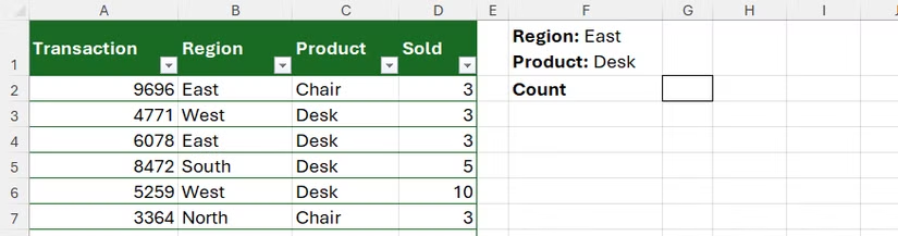
The formula will be written as follows:

=COUNTIFS(T_Sales[Region], "East", T_Sales[Product], "Desk")

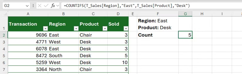
In this formula, "East" and "Desk" are criteria entered directly. While quick, this method lacks flexibility because you have to modify the formula every time you want to change a condition.

2. Optimization with cell references

A more efficient method is to place the criteria in separate cells and reference them in the formula. This allows for automatic updating of results when the values ​​in the criteria cells change.

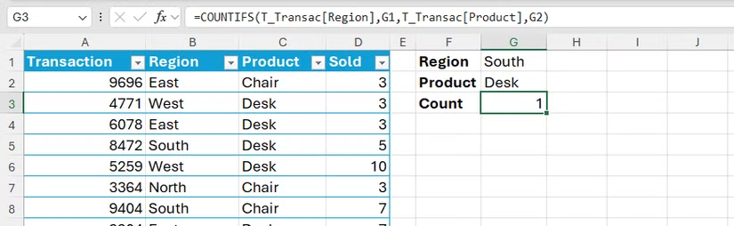
For example, to count the transactions in the tableT_TransacBased on the region and product entered in cells G1 and G2:

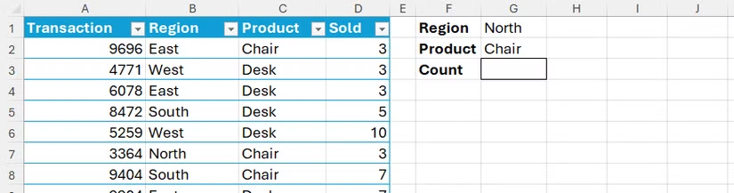
The formula in cell G3 will be:

=COUNTIFS(T_Transac[Region], G1, T_Transac[Product], G2)

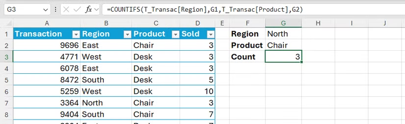
When you change the value in G1 or G2, the result will automatically update without needing to edit the formula.

3. Using comparison operators

When you need to count based on comparison conditions (greater than, less than, etc.), you need to combine the operator with a cell reference using an ampersand (&). For example, counting transactions in a table.T_TrackerThere is a transaction code greater than the value in cell G1 and a quantity sold greater than the value in cell G2.

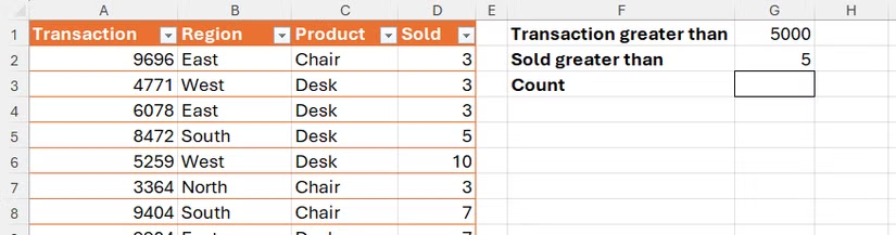
The formula needed:

=COUNTIFS(T_Tracker[Transaction], ">"&G1, T_Tracker[Sold], ">"&G2)

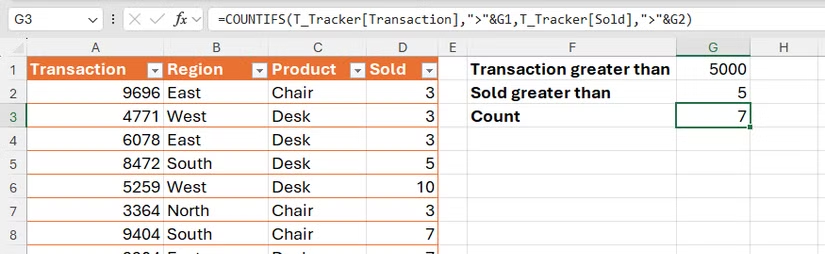
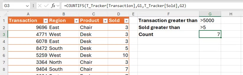
Comparison operators (e.g., ">") must be enclosed in double quotes and concatenated with the cell reference using the "&" character.

Advanced COUNTIFS techniques

1. Count the numbers in a range.

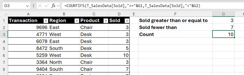
You can use COUNTIFS to count values ​​that lie between two boundaries by applying two conditions to the same data range. For example, count transactions in a table.T_SalesDataThe number of units sold is greater than or equal to the value in cell G1 and less than the value in cell G2.

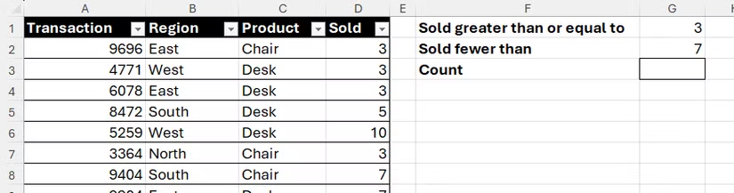
The formula is as follows:

=COUNTIFS(T_SalesData[Sold], ">="&G1, T_SalesData[Sold], "<"&G2)

2. OR logic simulation

To count items that satisfy one of several conditions (OR logic), you can add the results of several separate COUNTIFS functions. For example, count transactions from the area in cell G1 with a sales quantity at least equal to cell I1, OR transactions from area G2 with a sales quantity at least equal to cell I2.

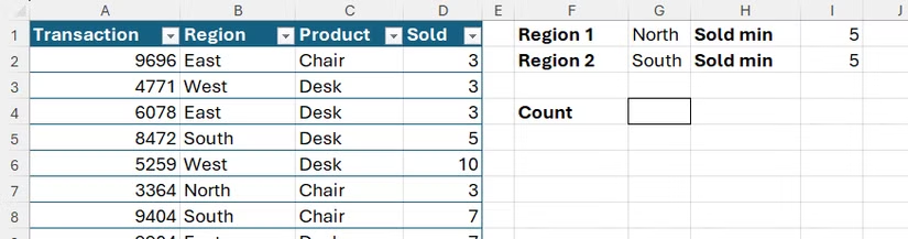
The formula will be the sum of the two COUNTIFS functions:

=COUNTIFS(T_Sales2025[Region], G1, T_Sales2025[Sold], ">="&I1) + COUNTIFS(T_Sales2025[Region], G2, T_Sales2025[Sold], ">="&I2)

3. Use wildcards

COUNTIFS supports wildcards for partial text searching:

• Star (*): Represents any string of characters.
• Question mark (?): Represents any single character.

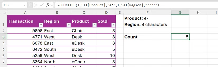
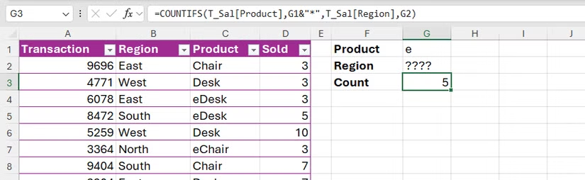
For example, count the transactions in the table.T_SalThe product name starts with "e" and the region name has exactly four characters.

The formula is needed:

=COUNTIFS(T_Sal[Product], "e*", T_Sal[Region], "????")

To make the formula more flexible, you can place wildcards in the cell references.

Conclude

The COUNTIFS function is an essential tool for anyone who frequently works with data in Excel. By mastering its syntax and applications, users can perform complex data analysis tasks quickly and accurately, thereby improving work efficiency and making more effective data-driven decisions. Knowledge of this function is also fundamental to understanding similar functions such as SUMIFS and AVERAGEIFS.