Excel Tip: Automatically color rows when a checkbox is selected.

Using checkboxes in Microsoft Excel is an effective way to track work progress and automate spreadsheets. By combining checkboxes with the Conditional Formatting feature, users can automatically color or change the formatting of an entire row of data as soon as the corresponding checkbox is selected.

This article will provide detailed instructions on how to implement this technique, applying it to checkboxes inserted directly into cells (in-cell checkboxes via tabs).InsertThis feature is currently available in Excel for Microsoft 365, Excel for the web, and the mobile apps.

Operating principle: The underlying logic behind the checkbox

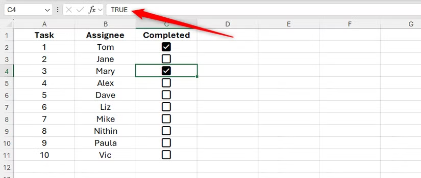
Before moving on to the formatting steps, it's important to understand how checkboxes work in Excel. When you insert a checkbox from the tab...InsertIt's not just a visual symbol. Each checkbox represents a Boolean logical value:

• Checked:Corresponding to the valueTRUE.
• Unchecked:Corresponding to the valueFALSE.

You can verify this by selecting a cell containing a checkbox and observing the value displayed in the formula bar. Understanding this mechanism is key to building formulas for conditional formatting.

Method 1: Formatting on a regular data range

This method applies to a standard range of cells, not formatted as an Excel Table. Let's say we have a to-do list with checkboxes in column C to mark completion.

The goal is that when a checkbox in column C is selected, the entire corresponding row (e.g., from column A to C) will be colored.

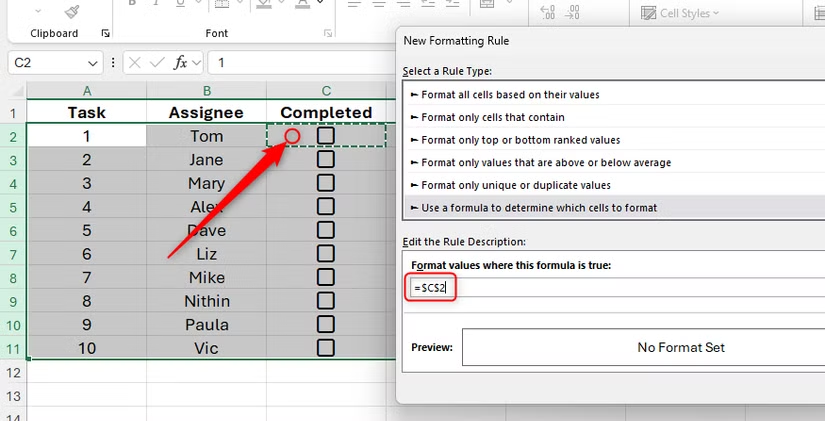
1. Select the data range:Select all the rows you want to apply the rule to. For example, drag your mouse from the header of row 2 to the end of row 11.
2. Open Conditional Formatting:On the tabGate, selectConditional Formatting > New Rule.
3. Choose the type of rule:In the new dialog box, select "Use a formula to determine which cells to format".
4. Enter the formula:In the formula cell, enter the following formula:=$C2=TRUE.
   Explanation of the formula:
   • =Start a recipe.
   • $C2This is a mixed reference. The dollar sign ($) before 'C' fixes column C, meaning the rule will always check the value in column C. The number '2' without the dollar sign is a relative reference, allowing the rule to automatically adjust to the following rows (e.g., $C3, $C4...).
   • =TRUEThe condition for the rule to be activated is when the checkbox in column C is selected.
5. Set the format:Click the buttonFormat, choose the background color, font style, or other formatting you want to apply (for example, strikethrough text).
6. Completed:ClickOKPress twice to close the dialog boxes and apply the rule.

Now, every time you check a cell in column C, the entire row will automatically change its formatting.

Advantages and disadvantages of this method

• Advantage:If you select the entire row (instead of just the data range), the formatting will automatically apply to the newly added columns to the right.
• Disadvantages:Applying formatting to entire rows can reduce Excel's performance, especially with large spreadsheets. Additionally, when you add data to new rows immediately below, you have to manually update the rule's scope in the settings.manage Rules.

Method 2: Optimization with Excel Tables

Use an Excel spreadsheet (created by selecting data and pressing Enter).Ctrl + T) offers many benefits, especially the ability to automatically expand formatting and formulas for new rows.

The steps are similar to the method above, but there are a few key differences:

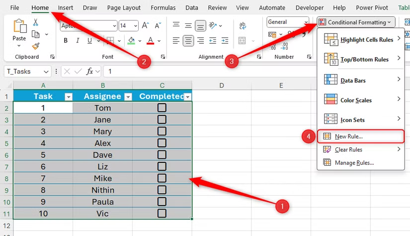
1. Select the data range in the table:Select all the cells in the table that you want to format (except the header row).
2. Create a new rule:AccessHome > Conditional Formatting > New Rule.
3. Enter the formula:Use the same mixed reference formula:=$C2=TRUE(Assuming the first active cell in the selection is A2 and the checkbox is in column C).
4. Apply the formatting and you're done.

Advantages and disadvantages of using Excel spreadsheets.

• Advantage:The biggest benefit is that when you add a new row of data to the end of the table, conditional formatting is automatically applied. This saves time and prevents errors. Furthermore, the formatting only applies within the table, making Excel more efficient.
• Disadvantages:If you add a new column to the right of the table, you will have to go tomanage Rulesto expand the scope of application for that new column.

In summary, combining checkboxes and conditional formatting is a powerful technique that transforms Excel spreadsheets from static data entry tools into intuitive and automated management systems. Depending on your data structure, you can choose to use regular ranges or Excel tables for optimal results.